NKI_statistics

This website is provided by the NKI Biostatistics Center (here) and supports researchers conducting mice experiments at the Netherlands Cancer Institute in the statistical aspects of the studies. It provides explanations of basic statistical concepts and tests. Moreover, researchers can use this app to calculate the required sample size when an experiment is being designed. The latter is vital and must be performed, because :

More power increases the confidence in the results, whether they are significant or not

Some background about sample size calculations can be found in the Statistical Power section

Sample size calculation depends on the type of experiment. In most of the mouse experiments conducted in the Netherlands Cancer Institute, groups of mice are compared with respect to mean/median values, survival outcomes, proportions and tumor growth. Examples of such experiments are listed below and more information can be found under the specific tabs.

Comparison of means/medians

Example: : A scientist wants to test the hypothesis that a novel compound is superior in reducing high-density lipoprotein (HDL) cholesterol levels in a transgenic C57Bl/6J strain of mice in comparison to a standard treatment. In the experiment, one group of mice receives the standard treatment and the other group receives the novel compound. At the end of the experiment, the HDL cholesterol levels are determined in all mice and the average HDL cholesterol level between both groups is compared.

Go to Means/Median Analysis

Survival Analysis

Example: To evaluate whether the chemotherapeutic agent paclitaxel improves survival after esophageal adenocarcinoma (EAC), a scientist uses a peritoneal dissemination xenograft mouse model and injects human EAC cell lines intraperitoneally into severe combined immunodeficiency (SCID) mice. Two weeks later, the mice are randomly assigned to either vehicle or paclitaxel (20mg/kg, 2 times a week for 2 weeks) groups. Mice are followed until death or the end of the study duration to compare the survival distributions between the two groups.

Go to Survival Analysis

Proportion Analysis

Example: A scientist wants to test the hypothesis that a new combination treatment is associated with a higher proportion of mice having a complete response compared with a standard treatment. Mice without palpable tumors for 14 days are considered complete responders. The proportions of complete responders are compared between treatment groups.

Go to Proportion Analysis

Growth Curve Analysis

Example: A scientist wants to test the hypothesis that a new treatment is able to slow down tumor growth. An experiment is conducted where tumor cells are injected into mice and volume of the tumor is measured every 2-3 days. When tumors reach a pre-defined volume of 1500 mm3, mice are randomized to receive either the standard treatment or the new treatment. Tumor volume is measured until mice die or are sacrificed. The rate of tumor growth is compared between treatment groups.

Go to Growth Curve Analysis

An experiment is conducted to answer a particular research question, for instance, to investigate whether the outcome after a new treatment differs from the outcome after the standard treatment, i.e. whether there is an effect of the new treatment. The research question is typically framed into a null hypothesis (e.g., there is no treatment effect) and an alternative hypothesis (e.g., there is a treatment effect). The answer to the research question is based on a statistical hypothesis test, which either leads to the rejection of the null hypothesis or not. The statistical test is designed to generally reflect the true state of nature, but there is a chance for erroneous decisions. A researcher can make two types of correct decisions and two types of errors, which is shown in the table below.

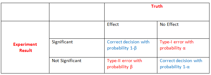
The effect either exists or not in nature, while the result of the statistical analysis is either significant or non-significant. Therefore, based on the statistical analysis, a researcher either makes a correct inference about the effect or a false one. The type 1 error ($\alpha$) is the probability of finding an effect, i.e. rejecting the null hypothesis of no effect, when it does not exist. It is also called the significance level of a test. The type 2 error ($\beta$) is the probability of not finding an effect, i.e., not rejecting the null hypothesis of no effect, when the effect exists. The type 1 error is the probability of a false positive finding, while the type 2 error is the probability of a false negative finding. Complements of the two probabilities, 1-$\alpha$ and 1-$\beta$ , are probabilities of correctly not finding an effect (true negative finding) and correctly finding an effect (true positive finding), respectively. The latter probability, 1- $\beta$, is also called the statistical power of a test. The value of $\alpha$ is usually fixed at 0.05. The value of beta decreases with increasing effect size and sample size.

If there is a true effect of a treatment, researchers would like to detect it with high probability. A power level of 0.8 or 0.9 is usually considered sufficient. For illustration, if 100 experiments are conducted with an existing true effect and each experiment has a power of 0.8 (i.e., 80%), the statistical analyses would be significant for 80 experiments (and result in rejection of the hypothesis of no effect), while 20 experiments would yield a non-significant result of the statistical test, i.e., the true effect would be missed (false negative finding). On the other hand, if none of the 100 experiments is based on a true effect, and a significance level of $\alpha$=0.05 (i.e., 5%) is used, then the statistical analysis of 5 experiments would be expected to be statistically significant (p<0.05), i.e., reflecting false positive (or chance) findings.

Statistical power is a measure of confidence to detect an effect (i.e., a significant result) if it truly exists. The power depends on the sample size of an experiment and the magnitude of the effect. During the design phase of an experiment, a researcher can assess how many mice need to be included in order to detect a true effect with sufficient probability. This assessment is important because an underpowered experiment (too few mice) can miss an effect that truly exists. An overpowered experiment (too many mice) can detect an effect that truly exists but is so small that it is not of practical relevance. In both situations, resources spent on an experiment, such as money, time or animals' lives are wasted.

* More power increases the chance of a significant result.
* More power increases the chance of replicating prior findings, if true.
* More power increases the confidence about the results, either significant or not.

So far, we assumed that a true effect does or does not exist. In reality, this is unknown. Let R be the probability that a true effect exists for a particular experiment or, in a large number of experiments (e.g., all experiments done in a career), the proportion of experiments with a true effect. The table of possible decisions based on statistical tests is then given by:

Assume a scientist develops and tests hypotheses so that a true effect exists (i.e., the null hypothesis is wrong) for half of her experiments (R=0.5). If she chooses the sample sizes of 100 experiments so that power is 80%, she is expected to obtain significant tests for 40 of the 50 experiments with a true effect (i.e., reject 40 of the 50 wrong null hypotheses) and miss the effect for the remaining 10 experiments (i.e., not reject 10 of the 50 wrong null hypotheses). If power is 50%, only 25 of the 50 true effects will, on average, be identified. For each experiment, four important measures are considered:

1.$$\text{True positive rate} = \frac{Power*R}{Power*R + (1-Power)*R} = Power$$The probability of a significant result if the effect truly exists.

2.$$\text{True negative rate} = \frac{(1-\alpha)*(1-R)}{(1-\alpha)*(1-R) + \alpha*(1-R)} = 1-\alpha$$The probability of a non-significant result if the effect does not exist. It is the complement of the type 1 error $\alpha$.

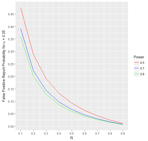
3.$$\text{Positive predictive value(PPV)} = \frac{Power*R}{Power*R + \alpha*(1-R)}$$The probability that the effect exists given a significant result of the statistical test. As can be seen from the formula and the graph below, this probability increases with increasing power and R.

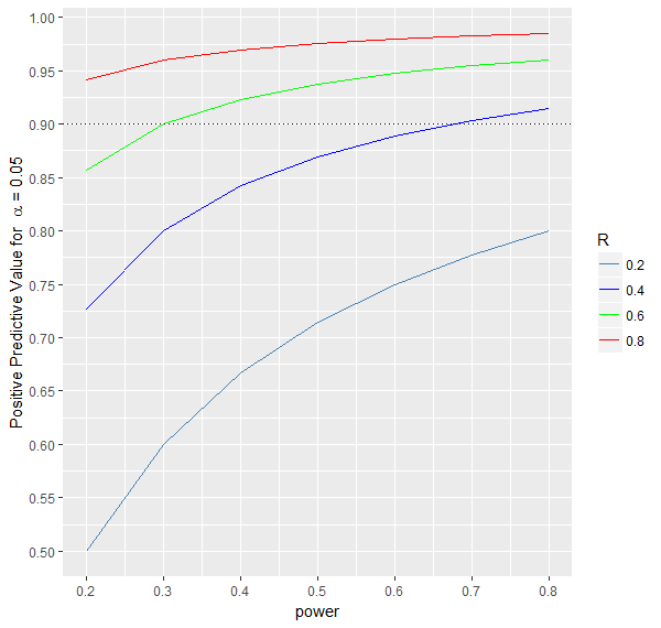
4.$$\text{False Positive Report Probability(FPRP)} = 1-PPV = \frac{\alpha*(1-R)}{Power*R + \alpha*(1-R)}$$The probability that there is no effect if the statistical test is significant. As can be seen from the formula and the graph below, this probability decreases with increasing power and R.

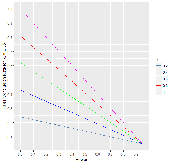
A false conclusion is either making a type 1 or type 2 error. The false conclusion rate can be determined by combining the type 1 and type 2 errors. As is illustrated in the graph below, this rate decreases with increasing power and decreasing R. Moreover, when the prior probability of the effect is maximum, i.e., R=1, then the false conclusion rate depends only on the power of the test. More precisely, it is actually equal to the type 2 error $\beta$ or equivalently to 1-power. When R = 0, the false conclusion rate is equal to the type 1 error $\alpha$ . For fixed values of $\alpha$ and power, a higher probability R is associated with more false conclusions. The lower the power, the higher the influence of R on the false conclusion rate.

Statistical power depends on three factors

To determine the power of an analysis we need firstly to specify the alternative hypothesis, $H_a$, or in other words, the effect size that we are interested in detecting. Further, and for most of analyses, power is proportional to the following:

*Effect size : the size of the effect, which can be measured as a difference in mean/median values, survival outcomes, proportions or growth rates; the bigger the effect size the higher the power

*Sample size : the number of mice included in an experiment; the higher the number of mice the higher the power.

*Significance level($\alpha$) : the type 1 error of a test; the higher the $\alpha$ the higher the power, but $\alpha$ is almost always fixed at 0.05.

Power can be calculated based on the three factors. More often, the required sample size is calculated as a function of power, $\alpha$ and an estimate of the effect size. Sample size can be calculated for any study design and statistical test.

The correct sample size can be obtained through the following steps:

1. Formulate the research question, i.e., define clearly what the null hypothesis and the alternative hypothesis of interest are

2. Identify the statistical test to be performed on the data from the experiment

3. Determine a reasonable value for the expected effect size based on substantive knowledge, literature, previous experiments, or select the smallest effect size that is considered as clinically important

4. Select the desired $\alpha$ level (almost always 0.05)

5. Select the desired power level (mostly 0.8 or 0.9) and calculate the required sample size

Other tabs and links to external sources on this website allow you to calculate the sample size needed in different situations.

Multiple Comparisons

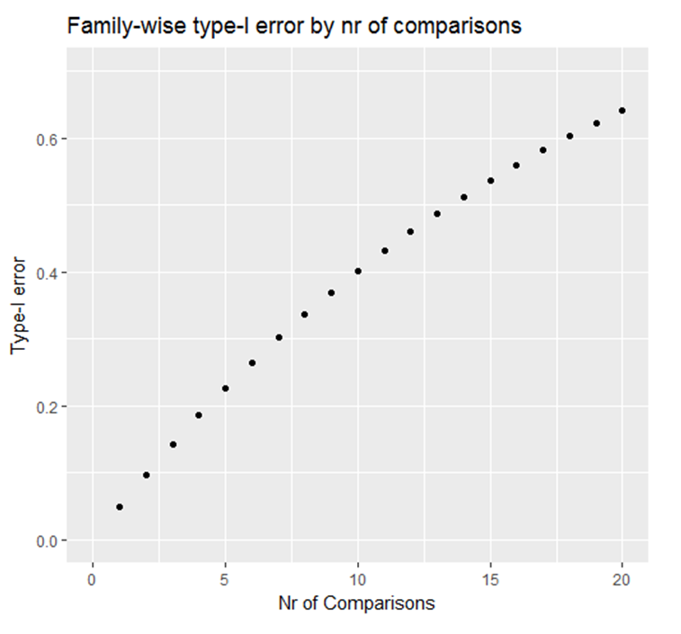
When an experiment involves more than one comparison, i.e., more than one null hypothesis and therefore more than one statistical test, the overall conclusion is that a subset of null hypotheses is rejected. For each test, the probability of a type 1 error is $\alpha$, but for all tests combined, the probability of a type 1 error is higher. This overall probability is also called the family-wise error rate or experiment-wise error rate. It is the probability that at least one comparison leads to a false positive finding and is calculated as: $$1-(1 - a)^{m}$$
where $\alpha$ is the significance level for an individual comparison and m is the total number of comparisons in the experiment. For instance, an experiment with 4 groups involves 6 pairwise comparisons. The probability that at least one comparison leads to a false-positive conclusion is equal to , $$1-(1 - 0.05)^{6} = .265$$
Many statistical techniques have been developed in order to deal with this issue, i.e., to control the family-wise error rate. The most common approach is the Bonferroni correction: the overall desired family-wise error rate (e.g., 0.05) is divided by the number of comparisons m in the experiment to find the individual $\alpha$ level to be used for each comparison. So, if a researcher wants to conduct m=10 statistical tests with a family-wise error rate of 0.05, the significance level for each individual test should be 0.05/10=0.005. This means that only those comparisons with P < 0.005 are considered significant and the probability that even one of the rejected hypotheses is a false-positive is less than 0.05.The control of the family-wise error needs to be taken into account not only in the data analysis phase of an experiment but also when sample size calculations are performed.

More information about the Bonferroni method can be found here

One-sided vs two-sided tests

Consider the example of a group of mice with food ad libitum and another group of similar mice with a severely restricted diet. A test comparing mean weight gain in the ad libitum group($\mu_{1}$) with that in the restricted group($\mu_{2}$) evaluates the null hypothesis that $\mu_{1}$=$\mu_{2}$. The alternative hypothesis could be $\mu_{1}$ $\neq$ $\mu_{2}$ (two-sided) or $\mu_{1}$>$\mu_{2}$ (one-sided) or $\mu_{2}$>$\mu_{1}$ (one-sided). A two-tailed test is appropriate if a difference between groups in both directions is possible and of interest. For instance, the comparison of two cancer treatments can show an effect in both directions, i.e., treatment A is better than treatment B or treatment B is better than treatment A. A one-tailed test is appropriate if a difference between groups is only possible in one direction and is practically impossible in the other direction. In the above weight gain example, a one-sided alternative of $\mu_{1}$>$\mu_{2}$ appears appropriate. In clinical research, one-sided tests are rarely appropriate.

More information about one and two sided tests can be found here

REFERENCES

The p value and the base rate fallacy

Scientific method: Statistical errors

The fickle P value generates irreproducible results

Observed power, and what to do if your editor asks for post-hoc power analyses

Statistical considerations for preclinical studies

A biologist's guide to statistical thinking and analysis

There are 2 free softwares that are widely used for sample size calculations.

G*Power

PS: Power and Sample Size Calculation

T-test and Mann-Whitney-Wilcoxon tests compare the mean or median of an outcome variable between two groups while ANOVA and Kruskal-Wallis test compare more than two groups. T-test and ANOVA are parametric tests that rely on certain distributional assumptions to obtain reliable test results. Validation of these assumptions becomes impossible when group sizes are small, which is the case with most animal experiments. Then, non-parametric tests should be used instead, namely Mann-Whitney-Wilcoxon or Kruskal-Wallis tests.

In an experiment with more than two groups of mice, the Kruskal-Wallis test indicates if at least one group differs from others (heterogeneity). To find the groups which differ, pairwise comparisons can be performed using Mann-Whitney-Wilcoxon tests. However, conducting multiple pairwise tests increases the overall probability of a false positive result (type 1 error), see Multiple Comparisons.To control this type 1 error at sufficient statistical power, a larger sample size is needed.

More information about the Mann-Whitney-Wilcoxon test can be found here

For 2 groups

A scientist wants to test the hypothesis that a novel compound reduces high-density lipoprotein (HDL) cholesterol levels in a transgenic C57Bl/6J strain of mice. Therefore, a new study is planned where mice will be randomized to a control and a treatment group, in order to compare the average HDL cholesterol levels between both groups. In an experiment, the following measurements of HDL were observed:

Analysis of such data can be carried out using the GraphPad software and following the steps described here

The following information from these data can be used to calculate the required sample size for a new experiment:

Mean HDL in control group
Mean HDL in treatment group
Standard deviation HDL in control group
Standard deviation HDL in treatment group

For more than 2 groups

A scientist wants to test the hypothesis that two novel compounds reduce high-density lipoprotein (HDL) cholesterol levels in a transgenic C57Bl/6J strain of mice. Therefore a new study is planned where mice will be randomized to the two treatment groups and an untreated group, in order to compare the average HDL cholesterol levels between the three groups. During an experiment, the following measurements of HDL are observed:

For an experiment with more than two groups, the required sample size can be calculated using information about the two groups with the smallest difference between the average outcome, i.e., HDL. If an experiment is powered for the smallest difference, it is also powered to detect a larger difference, but multiple comparisons should be taken into account (see Multiple Comparisons).

Usually, a control group is also included in the experiment. If the controls are only technical controls and not of direct interest, it is not necessary to include them as a group in the analysis and in the adjustment of the type 1 error.

Sample size calculation Example

Calculations of the required sample size can be performed under the Sample Size Calculation tab. For illustration, we will use the examples described above.

For 2 groups

For this particular example, we have:

Mean HDL in treatment group = 267.39
Mean HDL in control group = 283.46
Standard Deviation HDL in treatment group = 14.38
Standard Deviation HDL in control group = 11.83

For such an experiment the required sample size is 14 per group.

For more than 2 groups

For this particular example, we have:

Mean HDL in treatment group A = 267.39
Mean HDL in treatment group B = 256.48
Mean HDL in treatment group C = 283.46
Standard Deviation HDL in treatment group A = 14.83
Standard Deviation HDL in treatment group B = 9.75
Standard Deviation HDL in treatment group C = 11.83

The smallest difference in outcome is between groups A and B. Since three pairwise tests will be performed, an $\alpha$ value of 0.05/3 = 0.0166 is used.

For such an experiment the required sample size is 31 per group.

Information on how to use this online calculator is provided in the Example. This is a simulation based calculation and therefore it might take few seconds depending on the input.

Means for group A and B are assumed to be and respectively, while standard deviations are for group A and for group B. To detect the population mean difference of M1-M2 = with an $\alpha$ of % and % power based on a Mann-Whitney-Wilcoxon test, the required sample size per group is:

The log-rank test is used to test the null hypothesis that the time to an event (e.g., death or a tumor exceeding a pre-defined volume) between groups of mice is equal. For each mouse, the survival time is measured from the start of the experiment, for example from the time of randomization, until the mouse experiences the outcome of interest or is sacrificed or the experiment ends. For mice that do not experience the outcome during the study duration, the time to the outcome event is unknown and therefore their survival time is censored. The log-rank test compares differences in survival time based on the hazard ratio as a measure of effect size. The hazard ratio equals the ratio of the median survival times in both groups for exponential survival distributions.

Here , you can find more information about the log-rank test.

To evaluate whether the chemotherapeutic agent paclitaxel improves survival after esophageal adenocarcinoma (EAC), a scientist uses a peritoneal dissemination xenograft mouse model and injects human EAC cell lines intraperitoneally into severe combined immunodeficiency (SCID) mice. Two weeks later, the mice are randomly assigned to either vehicle or paclitaxel (20mg/kg, 2 times a week for 2 weeks) groups. Mice are followed until death or the end of the study duration to compare the survival distributions between the two groups.

Analysis of such data can be carried out using the GraphPad software and following the steps described here

To calculate the sample size for a new experiment the following information is needed:

Median survival time in the control group
Median survival time in the treatment group
Duration of the experiment
Power level
Significance level

Sample size calculation example

Calculations of the required sample size can be performed using this website under the sample size calculation tab. For illustration, we will use the example described above.

For this particular example, we have:

Median Survival in the control group = 18.5 days
Median Survival in the treatment group = 40.5 days
Duration of the experiment = 60 days

Information on how to use this online calculator is provided in the Example

The median survival time of the control group is expected to be days and the total duration of the experiment is assumed to be days. To detect the ratio between the median survival time of the treatment group to control group of with an $\alpha$ of % and % power based on a logrank test, the required sample size per group is:

When the outcome is binary, the comparison of groups is a comparison of proportions. For example, after treatment, mice can have a complete response (coded as 1) or not complete response (coded as 0). This situation can be analyzed with a Z-test comparing the proportions of responding mice between two different treatments. But because of the small sample sizes that are usually used in mice experiments, it is more appropriate to use Fisher's exact test

More information about the Z-test for proportions can be found here and about the Fisher's exact test here

A scientist wants to test the hypothesis that a new combination treatment leads to a higher proportion of tumor regression compared with a standard treatment . Mice that do not have palpable tumors for 14 days are considered responders. The proportions of responders are compared between treatment groups. The data from an experiment are presented below.

Analysis of such data can be carried out using the GraphPad software and following the steps described here.

To calculate the required sample size for a new similar experiment, the proportions of responding mice in control and treatment group need to be estimated from that data.

Sample Size calculation example

Calculations of the required sample size can be performed under the Sample Size Calculation tab. For illustration, we will use the example described above.

Proportion responders after standard treatment = 10%
Proportion responders after new combination treatment = 30%

Information on how to use this online calculator is provided in the Example. This is a simulation based calculation and therefore it might take a few seconds depending on the input.

The proportions in two groups are expected to be and . To detect the difference between these proportions of with an $\alpha$ of % and % power based on , the required sample size per group is:

In this type of experiments, tumor cells are injected into mice and the volume of the tumor is measured every 2-3 days. When the tumor reaches a certain volume, e.g. $200mm^3$, mice are randomized into treatment and control groups. Tumor volume is regularly measured until mice die or are sacrificed. The objective is to compare the tumor growth between groups. Often, average tumor size is compared at arbitrary time points using a T-test or ANOVA.This approach is inappropriate. A proper test if tumor growth rates differ between groups should be based on a linear regression which uses all measured tumor volumes for each mouse and accounts for the correlation between observations from the same mouse. If the tumor volume measure does not follow a normal distribution, its transformed values should be used as the outcome in a linear regression. The most common transformation applied in such studies is the logarithmic transformation.

A scientist wants to test the hypothesis that a new treatment is able to suppress the tumor growth. An experiment is conducted where tumor cells are injected into mice and volume of the tumor is measured every 2-3 days. When tumors reach a pre-defined volume of $1500mm^3$, mice are randomized to receive either the standard treatment or the new treatment. Tumor volume is measured until mice die or are sacrificed in order to compare the rate of tumor growth between treatment groups.

The data from an experiment are presented below. The NA denotes an unmeasured volume for mice that died or were sacrificed before the end of the study duration.

Such data cannot be analyzed with Graphpad software, but SPSS software can be used instead. Installation of SPSS software can be requested from the IT department free of charge for NKI employees.

Data in a long format should be loaded in SPSS. In such data format, each row corresponds to one measurement per mouse and there are as many rows per mouse as there are volume measurements available.

1. Loading data into SPSS: File -> Open -> Data

2. Creating a binary indicator variable ‘TreatmentGR’ with values 0 for control group and 1 for treatment group:

Transform -> Compute Variable -> Target Variable: TreatmentGR ; Numeric Expression : 0 -> If -> Include if case satisfies condition : Treatment = 'Control';

Transform -> Compute Variable -> Target Variable: TreatmentGR ; Numeric Expression : 1 -> If -> Include if case satisfies condition : Treatment = 'anti-PD1'

Screenshots below show how to do it for the control group.

3. Creating a variable ‘Days_TreatmentGr’ for the interaction between time (variable 'days') and treatment (variable 'TreatmentGR'):

Transform -> Compute Variable -> Target Variable: Days_TreatmentGr; Numeric Expression: Days*TreatmentGr

4. Performing a linear regression that accounts for the correlation between observations from the same mouse:

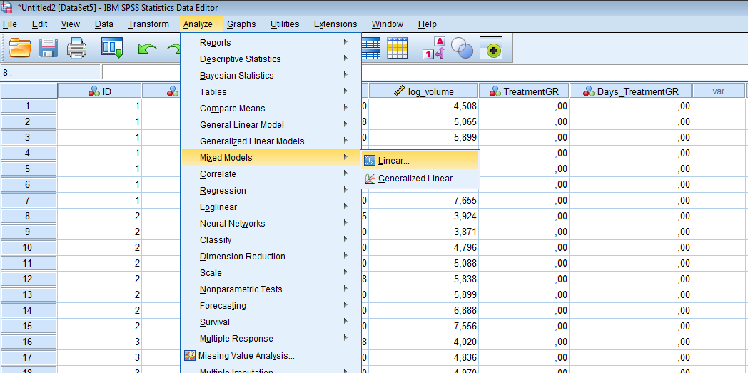
Analyze -> Mixed Models -> Linear... -> Subjects: ID; Repeated: days; Repeated Covariance Type: AR(1) -> Continue -> Dependent Variable : log_volume; Covariate(s): days, Days_TreatmentGr -> Fixed -> Model: days, Days_TreatmentGr using Main Effects option -> Continue -> Statistics -> Model Statistics: Parameter estimates for fixed effects -> Continue.

5. Interpreting results of the analysis:

Slope of the tumor growth in the control group = 0.226 (estimate for variable ‘days’): in the control group tumor volume on the log scale increases each day by 0.226 Difference in the slope of the tumor growth between the control and treatment groups = -0.101 (estimate for variable ‘Days_TreatmentGR’): in the treatment group tumor volume on the log scale increases each day by 0.124 (0.226-0.101 = 0.124) Correlation between the closest two measurements within mice = 0.698 (estimate for ‘AR(1) rho’) Residual variance = 0.692 (estimate for ‘AR1 diagonal’)

6. Performing a linear regression that does not account for the correlation between observations from the same mouse:

Analyze -> Mixed Models -> Linear... -> Subjects: ID; Repeated: days; Repeated Covariance Type: Scale Identity -> Continue -> Dependent Variable : log_volume; Covariate(s): days, Days_TreatmentGr -> Fixed -> Model: days, Days_TreatmentGr using Main Effects option -> Continue -> Statistics -> Model Statistics: Parameter estimates for fixed effects -> Continue.

More details on how to conduct mixed-models analysis in SPSS can be found here

Sample size calculation example

The sample size required for this kind of experiment is computed from the sample size required for a simple linear regression multiplied by a factor called design effect. This factor corrects for the correlation between measurements from the same mouse. The design effect is defined as the ratio between the variance of the interaction term from a linear model that accounts for correlated measurements and the variance of the interaction term from a linear model that does not account for correlated measurements.

Calculations of the required sample size can be performed under the Sample Size Calculation tab. For illustration, we will use the example described above. As was already mentioned, this analysis should be done using the logarithmic transformation of the tumor volume as the response. For that reason the sample size calculation should be done using values on this scale and not the raw ones. Further, the number of measurements that will be used for this calculation should be realistic. It should reflect the number of measurements that is expected to be taken for each mouse. If many mice do not reach that number because of early death or sacrifice, then the sample size calculation would not be correct anymore.

Difference in tumor growth rates = -0.101
Variance of the residuals from the model that does not account for correlation = 0.636
Standard error of the interaction effect from the model that does not account for correlation = 0.0148
Standard error of the interaction effect from the model that accounts for correlation = 0.0249
Average number of measurements per mouse = 8
Time difference between two measurements = 2

The number of measurements used for the calculation is the expected number of observations per mouse.

Required number of mice for growth curve data is obtained by estimating required number of observations for a model that does not account for correlated measurements. Then the estimate is multiplied by a design factor (= variance of the interaction effect from the model that accounts for correlation / variance of the interaction effect from the model that does not account for correlation) and divided by the expected number of observations per mouse.

Information on how to use this online calculator is provided in the Example

The average number of measurements per mouse is and measurements are obtained approximately every time units. Standard errors of the interaction effect obtained with a linear regression that does and does not account for the correlated measurements are and , respectively. The ratio is the design effect, i.e., . To detect a difference in growth rates of with an $\alpha$ of % and % power, the required sample size per group is: